Pulse-level circuit simulation
This documentation page is adapted from the publication [1] under CC BY 4.0.
Overview
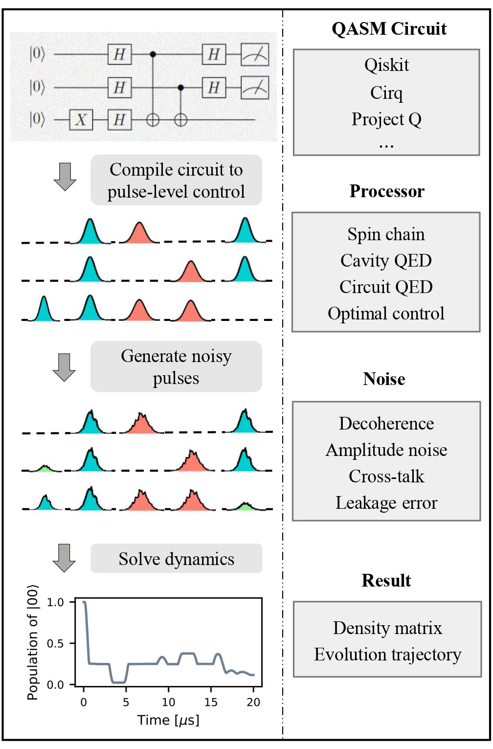
Based on the open system solver, Processor in the qutip_qip module simulates quantum circuits at the level of time evolution. One can consider the processor as an emulator of a quantum device, on which the quantum circuit is to be implemented.
The procedure is illustrated in the figure below. It first compiles the circuit into a Hamiltonian model, adds noisy dynamics and then uses the QuTiP open time evolution solvers to simulate the evolution.
In the following, we illustrate our framework with an example simulating a 3-qubit Deutsch-Jozsa algorithm on a chain of spin qubits. We will work through this example and explain briefly the workflow and all the main modules. .. testcode:
import numpy as np
from qutip import basis
from qutip_qip.circuit import QubitCircuit
from qutip_qip.device import LinearSpinChain

# Define a circuit
qc = QubitCircuit(3)
qc.add_gate("X", targets=2)
qc.add_gate("SNOT", targets=0)
qc.add_gate("SNOT", targets=1)
qc.add_gate("SNOT", targets=2)

# Oracle function f(x)
qc.add_gate("CNOT", controls=0, targets=2)
qc.add_gate("CNOT", controls=1, targets=2)

qc.add_gate("SNOT", targets=0)
qc.add_gate("SNOT", targets=1)

# Run gate-level simulation
init_state = basis([2,2,2], [0,0,0])
ideal_result = qc.run(init_state)

# Run pulse-level simulation
processor = LinearSpinChain(num_qubits=3, sx=0.25, t2=30)
processor.load_circuit(qc)
tlist = np.linspace(0, 20, 300)
result = processor.run_state(init_state, tlist=tlist)
In the above example, we first define a Deutsch-Jozsa circuit, and then run the simulation first at the gate-level.
We then choose the spin chain model for the underlying physical system, which is a subclass of Processor.
We provide the number of qubits and the \(\sigma_x\) drive strength 0.25MHz.
The other parameters, such as the interaction strength, are set to be the default value.
The decoherence noise can also be added by specifying the coherence times (\(T_1\) and \(T_2\)) which we discuss hereafter.
By initializing this processor with the hardware parameters, a Hamiltonian model for a spin chain system is generated, including the drift and control Hamiltonians.
The Hamiltonian model is represented by the Model class and is saved as an attribute of the initialized processor. In addition, the Processor can also hold simulation configurations such as whether to use a cubic spline interpolation for the pulse coefficients. Such configurations are not directly part of the model but nevertheless could be important for the pulse-level simulation.
Next, we provide the circuit to the processor through the method LinearSpinChain.load_circuit.
The processor will first decompose the gates in the circuit into native gates that can be implemented directly on the specified hardware model.
Each gate in the circuit is then mapped to the control coefficients and driving Hamiltonians according to the GateCompiler defined for a specific model.
A Scheduler is used to explore the possibility of executing several pulses in parallel.
With a pulse-level description of the circuit generated and saved in the processor, we can now run the simulation by
The Processor.run_state method first builds a Lindblad model including all the defined noise models (none in this example, but options are discussed below) and then calls a QuTiP solver to simulate the time evolution.
One can pass solver parameters as keyword arguments to the method, e.g., tlist (time sequence for intermediate results), e_ops (measurement observables) and options (solver options).
In the example above, we record the intermediate state at the time steps given by tlist.
The returned result is a Result object, which, depending on the solver options, contains the final state, intermediate states and the expectation value.
This allows one to extract all information that the solvers in QuTiP provide.
Theory
Down to the physical level, quantum hardware, on which a circuit is executed, is described by quantum theory. The dynamics of the system that realizes a unitary gate in quantum circuit is characterized by the time evolution of the quantum system. For isolated or open quantum systems, we consider both unitary time evolution and open quantum dynamics. The latter can be simulated either by solving the master equation or sampling Monte Carlo trajectories. Here, we briefly describe those methods as well as the corresponding solvers available in QuTiP.
For a closed quantum system, the dynamics is determined by the Hamiltonian and the initial state. From the perspective of controlling a quantum system, the Hamiltonian is divided into the non-controllable drift \(H_{\rm{d}}\) (which may be time dependent) and controllable terms combined as \(H_{\rm{c}}\) to give the full system Hamiltonian
where the \(H_j\) describe the effects of available physical controls on the system that can be modulated by the time-dependent control coefficients \(c_j(t)\), by which one drives the system to realize the desired unitary gates.
The unitary \(U\) that is applied to the quantum system driven by the Hamiltonian \(H(t)\) is a solution to the Schrödinger operator equation
By choosing \(H(t)\) that implements the desired unitaries (the quantum circuit) we obtain a pulse-level description of the circuit in the form of the control Hamiltonian. The choice of the solver depends on the parametrization of the control coefficients \(c_j(t)\). The parameters of \(c_j(t)\) may be determined through theoretical models or automated through control optimisation, as introduced later.
Processor and Model
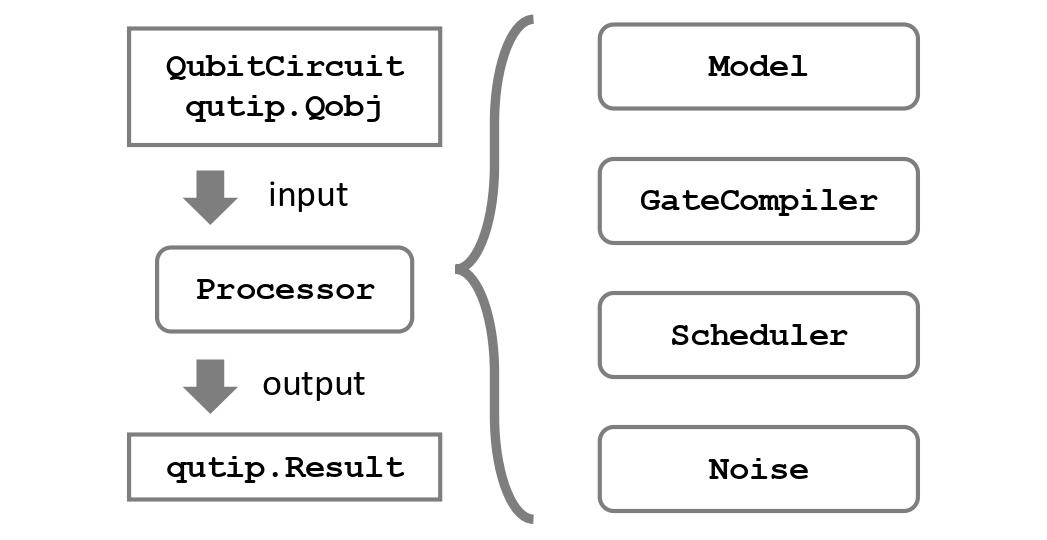
The Processor class handles the routine of a pulse-level simulation.
It connects different modules and works as the main API interface, as the figure below illustrates.
We provide a few predefined processors with Hamiltonian models and compilers routines. They differ mainly in how to find the control pulse for a quantum circuit, which gives birth to different sub-classes:
In general, there are two ways to find the control pulses. The first one, ModelProcessor, is more experiment-oriented and based on physical models. An initialized processor has a Processor.model attributes that save the control Hamiltonians. This is usually the case where control pulses realising those gates are well known and can be concatenated to realize the whole quantum circuits. Three realizations have already been implemented: the spin chain, the Cavity QED and the circuit QED model. In those models, the driving Hamiltonians are predefined, saved in the corresponding Model object. Another approach, based on the optimal control module in QuTiP, is called OptPulseProcessor. In this subclass, one only defines the available Hamiltonians in their system. The processor then uses algorithms to find the optimal control pulses that realize the desired unitary evolution.
Despite this difference, the logic behind all processors is the same:
One defines a processor by a list of available Hamiltonians and, as explained later, hardware-dependent noise. In model-based processors, the Hamiltonians are predefined and one only needs to give the device parameters like frequency and interaction strength.
The control pulse coefficients and time slices are either specified by the user or calculated by the method
Processor.load_circuit(), which takes aQubitCircuitand find the control pulse for this evolution.The processor calculates the evolution using the QuTiP solvers. Collapse operators can be added to simulate decoherence. The method
Processor.run_state()returns a objectResult.
It is also possible to calculate the evolution analytically with matrix exponentiation by setting analytical=True. A list of the matrices representing the gates is returned just like for QubitCircuit.propagators(). However, this does not consider the collapse operators or other noise. As the system size gets larger, this approach will become very inefficient.
In the following, we describe the predefined subclasses for Processor:
SpinChain
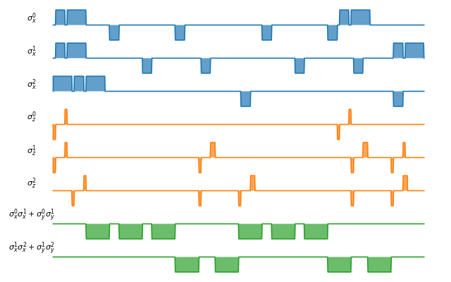
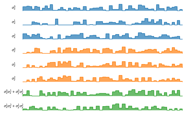
LinearSpinChain and CircularSpinChain are quantum computing models based on the spin chain realization. The control Hamiltonians are \(\sigma_x\), \(\sigma_z\) and \(\sigma_x \sigma_x + \sigma_y \sigma_y\). This processor will first decompose the gate into the universal gate set with ISWAP or SQRTISWAP as two-qubit gates, resolve them into quantum gates of adjacent qubits and then calculate the pulse coefficients.
In the following example we plot the compiled Deutsche Jozsa algorithm:
# Deutsch-Jozsa algorithm
from qutip_qip.circuit import QubitCircuit
qc = QubitCircuit(3)
qc.add_gate("X", targets=2)
qc.add_gate("SNOT", targets=0)
qc.add_gate("SNOT", targets=1)
qc.add_gate("SNOT", targets=2)

# Oracle function f(x)
qc.add_gate("CNOT", controls=0, targets=2)
qc.add_gate("CNOT", controls=1, targets=2)

qc.add_gate("SNOT", targets=0)
qc.add_gate("SNOT", targets=1)

from qutip_qip.device import LinearSpinChain
spinchain_processor = LinearSpinChain(num_qubits=3, t2=30)  # T2 = 30
spinchain_processor.load_circuit(qc)
fig, ax = spinchain_processor.plot_pulses(figsize=(8, 5))
fig.show()
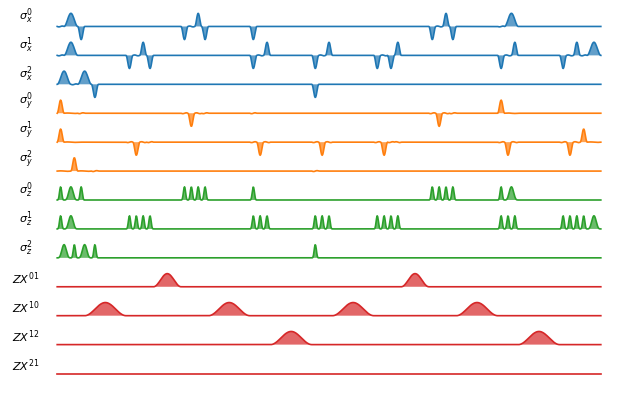
Superconducting qubits
For the SCQubits model, the qubit is simulated by a three-level system, where the qubit subspace is defined as the ground state and the first excited state.
The three-level representation will capture the leakage of the population out of the qubit subspace during single-qubit gates.
The single-qubit control is generated by two orthogonal quadratures \(a + a^{\dagger}\) and \(i(a - a^{\dagger})\), truncated to a three-level operator.
Same as the Spin Chain model, the superconducting qubits are aligned in a 1 D structure and the interaction is only possible between adjacent qubits.
As an example, the default interaction is implemented as a Cross Resonant pulse.
Parameters for the interaction strength are taken from [2][3].
from qutip_qip.device import SCQubits
scqubits_processor = SCQubits(num_qubits=3)
scqubits_processor.load_circuit(qc)
fig, ax = scqubits_processor.plot_pulses(figsize=(8, 5))
fig.show()
DispersiveCavityQED
Same as above, DispersiveCavityQED is a simulator based on Cavity Quantum Electrodynamics. The workflow is similar to the one for the spin chain, except that the component systems are a multi-level cavity and a qubits system. The control Hamiltonians are the single-qubit rotation together with the qubits-cavity interaction \(a^{\dagger} \sigma^{-} + a \sigma^{+}\). The device parameters include the cavity frequency, qubits frequency, detuning and interaction strength etc.
Note
The DispersiveCavityQED.run_state() method of DispersiveCavityQED
returns the full simulation result of the solver,
hence including the cavity.
To obtain the circuit result, one needs to first trace out the cavity state.
OptPulseProcessor
The OptPulseProcessor uses the function in optimize_pulse_unitary() in the optimal control module to find the control pulses. The Hamiltonian includes a drift part and a control part and only the control part will be optimized. The unitary evolution follows
To let it find the optimal pulses, we need to give the parameters for optimize_pulse_unitary() as keyword arguments to OptPulseProcessor.load_circuit(). Usually, the minimal requirements are the evolution time evo_time and the number of time slices num_tslots for each gate. Other parameters can also be given in the keyword arguments. For available choices, see optimize_pulse_unitary(). It is also possible to specify different parameters for different gates, as shown in the following example:
from qutip_qip.device import OptPulseProcessor, SpinChainModel
setting_args = {"SNOT": {"num_tslots": 6, "evo_time": 2},
                "X": {"num_tslots": 1, "evo_time": 0.5},
                "CNOT": {"num_tslots": 12, "evo_time": 5}}
opt_processor = OptPulseProcessor(
    num_qubits=3, model=SpinChainModel(3, setup="linear"))
opt_processor.load_circuit(  # Provide parameters for the algorithm
    qc, setting_args=setting_args, merge_gates=False,
    verbose=True, amp_ubound=5, amp_lbound=0)
fig, ax = opt_processor.plot_pulses(figsize=(8, 5))
fig.show()
Compiler and scheduler
Compiler
A compiler converts the quantum circuit to the corresponding pulse-level controls \(c_j(t)H_j\) on the quantum hardware.
In the framework, it is defined as an instance of the GateCompiler class.
The compilation procedure is achieved through the following steps.
First, each quantum gate is decomposed into the native gates (e.g., rotation over \(x\), \(y\) axes and the CNOT gate), using the existing decomposition scheme in QuTiP. If a gate acts on two qubits that are not physically connected, like in the chain model and superconducting qubit model, SWAP gates are added to match the topology before the decomposition. Currently, only 1-dimensional chain structures are supported.
Next, the compiler maps each quantum gate to a pulse-level control description. It takes the hardware parameter defined in the Hamiltonian model and computes the pulse duration and strength to implement the gate. A pulse scheduler is then used to explore the possibility of executing multiple quantum gates in parallel.
In the end, the compiler returns a time-dependent pulse coefficient \(c_j(t)\) for each control Hamiltonian \(H_j\). They contain the full information to implement the circuit and are saved in the processor. The coefficient \(c_j(t)\) is represented by two NumPy arrays, one for the control amplitude and the other for the time sequence. For a continuous pulse, a cubic spline is used to approximate the coefficient. This allows the use of compiled Cython code in QuTiP to achieve better performance.
For the predefined physical models described in the previous subsection, the corresponding compilers are also included and they will be used when calling the method Processor.load_circuit.
Note
It is expected that the output of the compiler will change after the official release of qutip-v5.
The use of the new Coefficient class will allow more flexibility and improve performance.
Therefore, we recommend to not parse the compiled result themselves but use Processor.set_tlist and Processor.set_coeffs instead.
Scheduler
The scheduling of a circuit consists of an important part of the compilation. Without it, the gates will be executed one by one and many qubits will be idling during the circuit execution, which increases the execution time and reduces the fidelity. In the framework, the scheduler is used after the control coefficient of each gate is computed. It runs a scheduling algorithm to determine the starting time of each gate while keeping the result correct.
The heuristic scheduling algorithm we provide offers two different modes: ASAP (as soon as possible) and ALAP (as late as possible). In addition, one can choose whether permutation among commuting gates is allowed to achieve a shorter execution time. The scheduler implemented here does not take the hardware architecture into consideration and assumes that the connectivity in the provided circuit matches with the hardware at this step.
In predefined processors, the scheduler runs automatically when loading a circuit and hence there is no action necessary from the side of the user.
Pulse shape
Apart from square pulses, compilers also support different pulse shapes.
All pulse shapes from SciPy window functions that do not require additional parameters are supported.
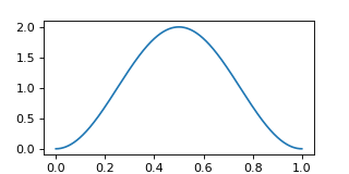
The method GateCompiler.generate_pulse_shape allows one to generate pulse shapes that fulfil the given maximum intensity and the total integral area.
from qutip_qip.compiler import GateCompiler
compiler = GateCompiler()
coeff, tlist = compiler.generate_pulse_shape(
    "hann", 1000, maximum=2., area=1.)
fig, ax = plt.subplots(figsize=(4,2))
ax.plot(tlist, coeff)
ax.set_xlabel("Time")
fig.show()
For predefined compilers, the compiled pulse shape can also be configured by the keyword "shape" and "num_samples" in the dictionary attribute GateCompiler.args
or the args parameter of GateCompiler.compile.
Noise Simulation
The Noise module allows one to add control and decoherence noise following the Lindblad description of open quantum systems.
Compared to the gate-based simulator, this provides a more practical and straightforward way to describe the noise.
In the current framework, noise can be added at different layers of the simulation, allowing one to focus on the dynamics of the dominant noise, while representing other noise, such as single-qubit relaxation, as collapse operators for efficiency.
Depending on the problem studied, one can devote the computing resources to the most relevant type of noise.
Apart from imperfections in the Hamiltonian model and circuit compilation, the Noise class in the current framework defines deviations of the real physical dynamics from the compiled one.
It takes the compiled pulse-level description of the circuit (see also Pulse representation) and adds noise elements to it, which allows defining noise that is correlated to the compiled pulses.
In the following, we detail the three different noise models already available in the current framework.
Noise in the hardware model
The Hamiltonian model defined in the Model class may contain intrinsic imperfections of the system and hence the compiled ideal pulse does not implement the ideal unitary gate.
Therefore, building a realistic Hamiltonian model usually already introduces noise to the simulation.
An example is the superconducting qubits, where the physical qubit is represented by a multi-level system.
Since the second excitation level is only weakly detuned from the qubit transition frequency, the population may leak out of the qubit subspace.
Another example is an always-on ZZ type cross-talk induced by interaction with higher levels of the physical qubits [4], which is also implemented for the superconducting qubit model.
Control noise
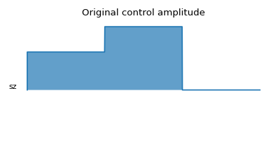
The control noise, as the name suggests, arises from imperfect control of the quantum system, such as distortion in the pulse amplitude or frequency drift. The simplest example is the random amplitude noise on the control coefficient \(c_j(t)\) in the control Hamiltonian.
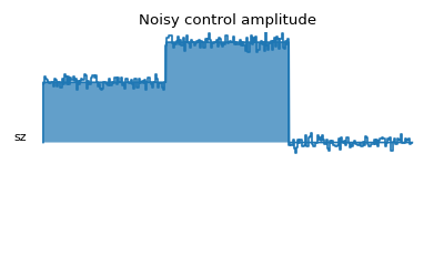
The following example demonstrates a biased Gaussian noise on the pulse amplitude. For visualization purposes, we plot the noisy pulse intensity instead of the state fidelity. The three pulses can, for example, be a zyz-decomposition of an arbitrary single-qubit gate:
from qutip import sigmaz, sigmay
from qutip_qip.device import Processor
from qutip_qip.noise import RandomNoise

# add control Hamiltonians
processor = Processor(1)
processor.add_control(sigmaz(), targets=0, label="sz")

# define pulse coefficients and tlist for all pulses
processor.set_coeffs({"sz": np.array([0.3, 0.5, 0. ])})
processor.set_tlist(np.array([0., np.pi/2., 2*np.pi/2, 3*np.pi/2]))

# define noise, loc and scale are keyword arguments for np.random.normal
gaussnoise = RandomNoise(
            dt=0.01, rand_gen=np.random.normal, loc=0.00, scale=0.02)
processor.add_noise(gaussnoise)

# Plot the ideal pulse
fig1, axis1 = processor.plot_pulses(
    title="Original control amplitude", figsize=(5,3),
    use_control_latex=False, dpi=200)

# Plot the noisy pulse
qobjevo, _ = processor.get_qobjevo(noisy=True)
fig2, axis2 = processor.plot_pulses(
    title="Noisy control amplitude", figsize=(5,3),
    use_control_latex=False, dpi=200)
tlist = np.linspace(0., processor.get_full_tlist()[-1], 300)
noisy_coeff = [qobjevo(t)[0, 0] for t in tlist]
axis2[0].step(tlist, noisy_coeff)
Lindblad noise
The Lindblad noise originates from the coupling of the quantum system with the environment (e.g., a thermal bath) and leads to loss of information. It is simulated by collapse operators and results in non-unitary dynamics [5][6].
The most commonly used type of Lindblad noise is decoherence, characterized by the coherence time \(T_1\) and \(T_2\) (dephasing).
For the sake of convenience, one only needs to provide the parameter t1, t2 to the processor and the corresponding operators will be generated automatically.
Both can be either a number that specifies one coherence time for all qubits or a list of numbers, each corresponding to one qubit.
For \(T_1\), the operator is defined as \(a/\sqrt{T_1}\) with \(a\) the destruction operator.
For \(T_2\), the operator is defined as \(a^{\dagger}a\sqrt{2/T_2^*}\), where \(T_2^*\) is the pure dephasing time given by \(1/T_2^*=1/T_2-1/(2T_1)\).
In the case of qubits, i.e., a two-level system, the destruction operator \(a\) is truncated to a two-level operator and is consistent with the Lindblad equation.
Constant \(T_1\) and \(T_2\) can be provided directly when initializing the Processor.
Custom collapse operators, including time-dependent ones, can be defined through DecoherenceNoise.
For instance, the following code defines a collapse operator using sigmam() and increases linearly as time:
from qutip_qip.device import LinearSpinChain
from qutip_qip.noise import DecoherenceNoise
tlist = np.linspace(0, 30., 100)
coeff = tlist * 0.01
noise = DecoherenceNoise(
    sigmam(), targets=0,
    coeff=coeff, tlist=tlist)
processor = LinearSpinChain(1)
processor.add_noise(noise)
Similar to the control noise, the Lindblad noise can also depend on the control coefficient.
Pulse representation
As discussed before, in this simulation framework, we compile the circuit into pulse-level controls and simulate the time evolution of the physical qubits. In this subsection, we describe how the dynamics is represented internally in the workflow, which is useful for understanding the simulation process as well as defining custom pulse-dependent noise.
A control pulse, together with the noise associated with it, is represented by a class instance of Pulse.
When an ideal control is compiled and returned to the processor, it is saved as an initialized Pulse, equivalent to the following code:
from qutip_qip.pulse import Pulse
coeff = np.array([1.])
tlist = np.array([0., np.pi])
pulse = Pulse(
    sigmax()/2, targets=0, tlist=tlist,
    coeff=coeff, label="pi-pulse")
This code defines a \(\pi\)-pulse implemented using the term \(\sigma_x\) in the Hamiltonian that flips the zeroth qubit specified by the argument targets. The pulse needs to be applied for the duration \(\pi\) specified by the variable tlist. The parameters coeff and tlist together describe the control coefficient.
Together with the provided Hamiltonian and target qubits, an instance of Pulse determines the dynamics of one control term.
Note
If the coefficients represent discrete pulse, the length of each array is 1 element shorter than tlist. If it is supposed to be a continuous function, the length should be the same as tlist.
With a Pulse initialized with the ideal control, one can define several types of noise, including the Lindblad or control noise as described in the noise section.
An example of adding a noisy Hamiltonian as control noise through the method Pulse.add_control_noise is given below:
pulse.add_control_noise(
    sigmaz(), targets=[0], tlist=tlist,
    coeff=coeff * 0.05)
The above code snippet adds a Hamiltonian term \(\sigma_z\), which can, for instance, be interpreted as a frequency drift.
Similarly, collapse operators depending on a specific control pulse can be added by the method Pulse.add_lindblad_noise.
In addition to a constant pulse, the control pulse and noise can also be provided as continuous functions. In this case, both tlist and coeff are given as NumPy arrays and a cubic spline is used to interpolate the continuous pulse coefficient.
This allows using the compiled Cython version of the QuTiP solvers that have a much better performance than using a Python function for the coefficient.
The option is provided as a keyword argument spline_kind="cubic" when initializing Pulse.
Similarly, the interpolation method can also be defined for Processor using the same signature.
Customize the simulator
As it is impractical to include every physical platform, we provide an interface that allows one to customize the simulators. In particular, the modular architecture allows one to conveniently overwrite existing modules for customization.
To define a customized hardware model, the minimal requirements are a set of available control Hamiltonians \(H_j\), and a compiler, i.e., the mapping between native gates and control coefficients \(c_j\).
One can either modify an existing subclass or write one from scratch by creating a subclass of the two parent classes Model and GateCompiler.
Since different subclasses share the same interface, different models and compilers can also be combined to build new processors.
Moreover, this customization is not limited to Hamiltonian models and compiler routines.
In principle, measurement can be defined as a customized quantum gate and the measurement statistics can be extracted from the obtained density matrix.
A new type of noise can also be implemented by defining a new Noise subclass, which takes the compiled ideal Pulse and adds noisy dynamics on top of it.
For examples, please refer to the tutorial notebooks.