Variational Quantum Algorithms

Implemented by Ben Braham as part of a Unitary Fund microgrant.

Overview

Variational Quantum Algorithms (VQAs) are a hybrid quantum-classical optimization algorithm in which an objective function (usually encoded by a parameterized quantum circuit) is evaluated by quantum computation, and the parameters of this function are updated using classical optimization methods. Such algorithms have been proposed for use in NISQ-era quantum computers as they typically scale well with the number of available qubits, and can function without high fault-tolerance.

In QuTiP, VQAs are represented by a parameterized quantum circuit, and include methods for defining a cost function for the circuit, and finding parameters that minimize this cost.

Constructing a VQA circuit

The VQA class allows for the construction of a parameterized circuit from VQABlock instances, which act as the gates of the circuit. In the most basic instance, a VQA should have:

Property	Description
num_qubits	Positive integer number of qubits for the circuit.
num_layers	Positive integer number of repetitions of the layered elements of the circuit.
cost_method	String referring to the method used to evaluate the circuit’s cost. Either “OBSERVABLE”, “BITSTRING”, or “STATE”.

For example:

from qutip_qip.vqa import VQA

VQA_circuit = VQA(
            num_qubits=1,
            num_layers=1,
            cost_method="OBSERVABLE",
        )

After constructing this instance, we are ready to begin adding elements to our parameterized circuit. Circuit elements in this module are represented by VQABlock instances. Fundamentally, the role of this class is to generate an operator for the circuit. To do this, it keeps track of its free parameters, and gives information to the VQA instance on how to update them. The operator itself can be generated by a user-defined function call, a parameterized Hamiltonian to exponentiate, a pre-computed unitary operator, or a string referring to a gate that has already been defined (either by the user already, or a gate native to QuTiP).

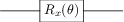
In the absence of specification, a VQA block takes a Qobj as the Hamiltonian \(H\), and will generate a unitary with free parameter, \(\theta\), as \(U(\theta) = e^{-i \theta H}\). For example,

from qutip_qip.vqa import VQA, VQABlock
from qutip import tensor, sigmax

VQA_circuit = VQA(num_qubits=1, num_layers=1)

R_x_block = VQABlock(
  sigmax() / 2, name="R_x(\\theta)"
)

VQA_circuit.add_block(R_x_block)

We added our block to the VQA_circuit with the VQA.add_block() method. Calling the VQA.export_image() method renders an image of our circuit in its current form:

---

Optimisation Loop

After specifying a cost method and function to the VQA instance, there are various options for optimization of the free circuit parameters. Calling VQA.optimize_parameters() will begin the optimization process and return an OptimizationResult instance. By default, the method will randomize initial parameters, and use the non-gradient-based COBYLA method for parameter optimization. Users can specify:

• Initial parameters. Given as a list, with length corresponding to the number of free parameters in the circuit. The number of free parameters can be computed automatically with the VQA.get_free_parameters_num() method. Alternatively, the string ‘zeros’ will initialize all parameters as 0; and ‘random’ will initialize parameters randomly between 0 and 1. Defaults to ‘random’.

• Optimization method. This can be a string referring to a pre-defined SciPy method listed here, or a callable function.

• Jacobian computation. A flag will tell the optimization method to compute the Jacobian at each step, which is passed to the optimizer so that it can use gradient information.

• Layer-by-layer training. Optimize parameters for the circuit with only a single layer, and hold these fixed while adding additional layers, up to VQA.num_layers.

• Bounds and constraints. To be passed to the optimizer.

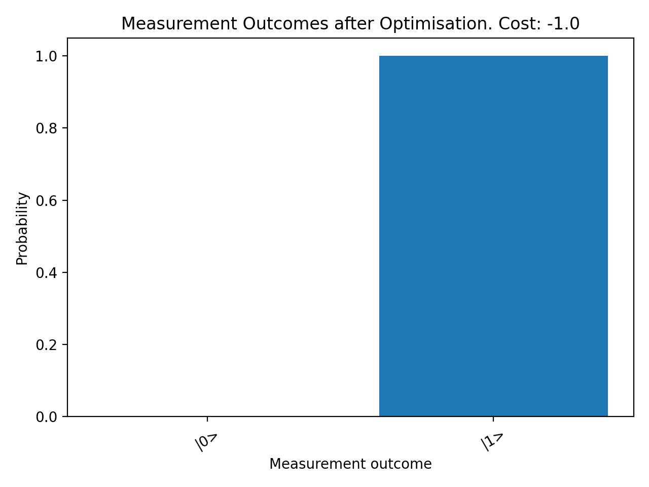
The OptimizationResult class provides information about the completed optimization process. For example, the probability amplitudes of different measurement outcomes of the circuit post-optimization can be plotted with OptimizationResult.plot().

Below, we run an optimization on a toy circuit, tuning a parameterized \(x\)-rotation gate to try to maximise the probability amplitude of the \(|1\rangle\) state.

>>> from qutip_qip.vqa import VQA, VQABlock
>>> from qutip import sigmax, sigmaz
>>> circ = VQA(num_qubits=1, cost_method="OBSERVABLE")

Picking the Pauli Z operator as our cost observable, our circuit’s cost function will be: \(\langle\psi(t)| \sigma_z | \psi(t)\rangle\)

>>> circ.cost_observable = sigmaz()

Adding a Pauli X operator as a block to the circuit, the operation of the entire circuit becomes: \(e^{-i t X /2}\).

>>> circ.add_block(VQABlock(sigmax() / 2))

We can now try to find a minimum in our cost function using the SciPy in-built L-BFGS-B (L-BFGS with box constraints) method. We specify the bounds so that our parameter is \(0 \leq t \leq 4\).

>>> result = circ.optimize_parameters(method="L-BFGS-B", use_jac=True, bounds=[[0, 4]])

Accessing result.res.x, we have the array of parameters found during optimization. In our case, we only had one free parameter, so we examine the first element of this array.

>>> angle = round(result.res.x[0], 2)
>>> print(f"Angle found: {angle}")
Angle found: 3.14

Finally, we can plot our the measurement outcome probabilities of our circuit after optimization.

>>> result.plot()

(png, hires.png, pdf)

(png, hires.png, pdf)

In this simple example, our optimization found that (neglecting phase) \(R_x(\pi) |0\rangle = |1\rangle\). Of course, this very basic usage generalizes to circuits on multiple qubits, with more complicated cost functions and optimization procedures.