Gate-level circuit simulation
Run a quantum circuit
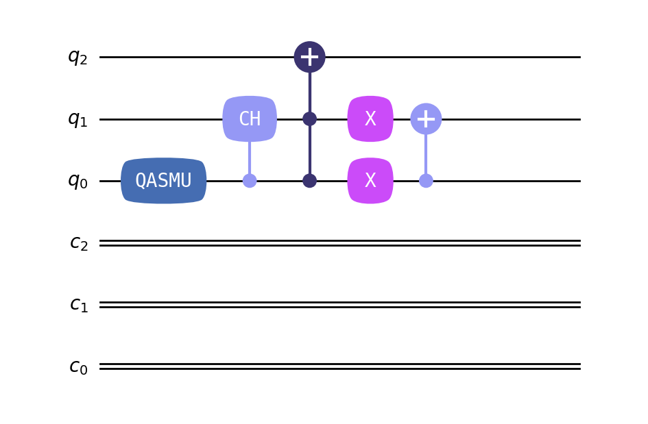
Let’s start off by defining a simple circuit which we use to demonstrate a few examples of circuit evolution. We take a circuit from OpenQASM 2
from qutip_qip.circuit import QubitCircuit
from qutip_qip.operations.gates import X, CX, CH, QASMU, TOFFOLI

qc = QubitCircuit(3, num_cbits=3)
qc.add_gate(QASMU, targets=[0], arg_value=[1.91063, 0, 0])
qc.add_gate(CH, controls=[0], targets=[1])
qc.add_gate(TOFFOLI, targets=[2], controls=[0, 1])
qc.add_gate(X, targets=[0])
qc.add_gate(X, targets=[1])
qc.add_gate(CX, targets=[1], controls=0)
qc.draw()
It corresponds to the following circuit:
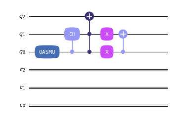
We will add the measurement gates later. This circuit prepares the W-state
\(\newcommand{\ket}[1]{\left|{#1}\right\rangle} (\ket{001} + \ket{010} + \ket{100})/\sqrt{3}\).
The simplest way to carry out state evolution through a quantum circuit is
providing an input state to the QubitCircuit.run() method.
from qutip import tensor, basis

zero_state = tensor(basis(2, 0), basis(2, 0), basis(2, 0))
result = qc.run(state=zero_state)
wstate = result

print(wstate)
Output:
Quantum object: dims=[[2, 2, 2], [1]], shape=(8, 1), type='ket', dtype=Dense
Qobj data =
[[0.     ]
 [0.57735]
 [0.57735]
 [0.     ]
 [0.57735]
 [0.     ]
 [0.     ]
 [0.     ]]
As expected, the state returned is indeed the required W-state.
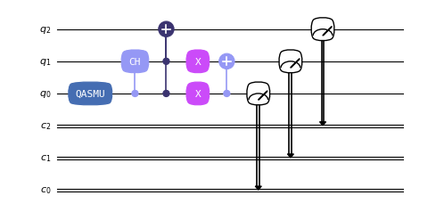
As soon as we introduce measurements into the circuit, it can lead to multiple outcomes with associated probabilities. We can also carry out circuit evolution in a manner such that it returns all the possible state outputs along with their corresponding probabilities. Suppose, in the previous circuit, we measure each of the three qubits at the end.
qc.add_measurement("M0", targets=[0], classical_store=0)
qc.add_measurement("M1", targets=[1], classical_store=1)
qc.add_measurement("M2", targets=[2], classical_store=2)
To get all the possible output states along with the respective probability of
observing the outputs, we can use the QubitCircuit.run_statistics()
function:
result = qc.run_statistics(state=tensor(basis(2, 0), basis(2, 0), basis(2, 0)))
states = result.get_final_states()
probabilities = result.get_probabilities()

for state, probability in zip(states, probabilities):
    print("State:\n{}\nwith probability {:.5f}".format(state, probability))
Output:
State:
Quantum object: dims=[[2, 2, 2], [1]], shape=(8, 1), type='ket', dtype=Dense
Qobj data =
[[0.]
 [1.]
 [0.]
 [0.]
 [0.]
 [0.]
 [0.]
 [0.]]
with probability 0.33333
State:
Quantum object: dims=[[2, 2, 2], [1]], shape=(8, 1), type='ket', dtype=Dense
Qobj data =
[[0.]
 [0.]
 [1.]
 [0.]
 [0.]
 [0.]
 [0.]
 [0.]]
with probability 0.33333
State:
Quantum object: dims=[[2, 2, 2], [1]], shape=(8, 1), type='ket', dtype=Dense
Qobj data =
[[0.]
 [0.]
 [0.]
 [0.]
 [1.]
 [0.]
 [0.]
 [0.]]
with probability 0.33333
The function returns a CircuitResult object which contains the output
states and their probabilities. The methods get_final_states()
and get_probabilities() can be used to obtain the possible
states and probabilities. Since the state created by the circuit is the W-state, we
\(\newcommand{\ket}[1]{\left|{#1}\right\rangle} \ket{001}\),
\(\newcommand{\ket}[1]{\left|{#1}\right\rangle} \ket{010}\) and
\(\newcommand{\ket}[1]{\left|{#1}\right\rangle} \ket{100}\)
with equal probability.
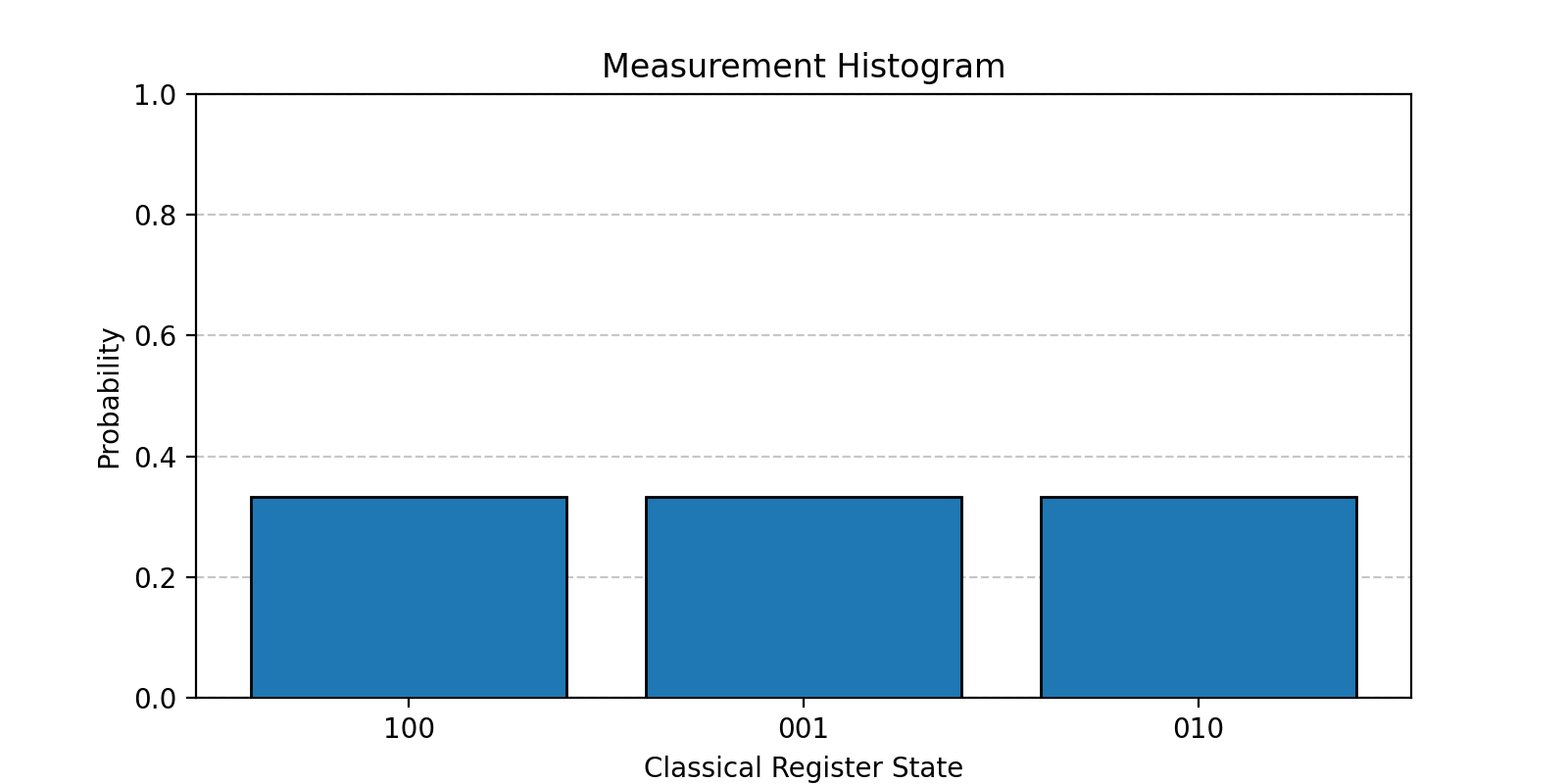
We can also visualize the measurement outcome probabilities using
plot_histogram():
import matplotlib.pyplot as plt

fig, ax = plt.subplots(figsize=(8, 4))
result.plot_histogram(fig=fig, ax=ax)

The histogram displays the probability of each classical register state. Since the W-state has equal probability of collapsing to \(\ket{001}\), \(\ket{010}\) and \(\ket{100}\), we observe each with probability \(1/3\).
Circuit simulator
The QubitCircuit.run() and QubitCircuit.run_statistics() functions
make use of the CircuitSimulator which enables exact simulation with
more granular options. The simulator object takes a quantum circuit as an argument.
It can optionally be supplied with an initial state. There are two modes in which
the exact simulator can function. The default mode is the
"state_vector_simulator" mode. In this mode, the state evolution proceeds
maintaining the ket state throughout the computation. For each measurement gate,
one of the possible outcomes is chosen probabilistically and computation proceeds.
To demonstrate, we continue with our previous circuit:
from qutip_qip.circuit import CircuitSimulator

sim = CircuitSimulator(qc)
sim.initialize(zero_state)
This initializes the simulator object and carries out any pre-computation
required. There are two ways to carry out state evolution with the simulator.
The primary way is to use the CircuitSimulator.run() and
CircuitSimulator.run_statistics() functions just like before (only
now with the CircuitSimulator class).
The CircuitSimulator class also enables stepping through the circuit:
sim.step()
print(sim.state)
Output:
Quantum object: dims=[[2, 2, 2], [1]], shape=(8, 1), type='ket', dtype=Dense
Qobj data =
[[0.57735]
 [0.     ]
 [0.     ]
 [0.     ]
 [0.8165 ]
 [0.     ]
 [0.     ]
 [0.     ]]
This only executes one gate in the circuit and allows for a better understanding of how the state evolution takes place. The method steps through both the gates and the measurements.
Density Matrix Simulation
By default, the state evolution is carried out in the
"state_vector_simulator" mode (specified by the mode argument) as
described before. In the "density_matrix_simulator" mode, the input state
can be either a ket or a density matrix. If it is a ket, it is converted into a
density matrix before the evolution is carried out. Unlike the
"state_vector_simulator" mode, upon measurement, the state does not collapse
to one of the post-measurement states. Rather, the new state is now the density
matrix representing the ensemble of post-measurement states. In this sense, we
measure the qubits and forget all the results.
To demonstrate this consider the original W-state preparation circuit which is followed just by measurement on the first qubit:
qc = QubitCircuit(3, num_cbits=3)
qc.add_gate(QASMU, targets=[0], arg_value=[1.91063, 0, 0])
qc.add_gate(CH, controls=[0], targets=[1])
qc.add_gate(TOFFOLI, targets=[2], controls=[0, 1])
qc.add_gate(X, targets=[0])
qc.add_gate(X, targets=[1])
qc.add_gate(CX, targets=[1], controls=0)
qc.add_measurement("M0", targets=[0], classical_store=0)
qc.add_measurement("M0", targets=[1], classical_store=0)
qc.add_measurement("M0", targets=[2], classical_store=0)
sim = CircuitSimulator(qc, mode="density_matrix_simulator")
print(sim.run(zero_state).get_final_states()[0])
Quantum object: dims=[[2, 2, 2], [2, 2, 2]], shape=(8, 8), type='oper', dtype=Dense, isherm=True
Qobj data =
[[0.      0.      0.      0.      0.      0.      0.      0.     ]
 [0.      0.33333 0.      0.      0.      0.      0.      0.     ]
 [0.      0.      0.33333 0.      0.      0.      0.      0.     ]
 [0.      0.      0.      0.      0.      0.      0.      0.     ]
 [0.      0.      0.      0.      0.33333 0.      0.      0.     ]
 [0.      0.      0.      0.      0.      0.      0.      0.     ]
 [0.      0.      0.      0.      0.      0.      0.      0.     ]
 [0.      0.      0.      0.      0.      0.      0.      0.     ]]
We are left with a mixed state.
Import and export quantum circuits
QuTiP supports importing and exporting quantum circuits in the
OpenQASM 2.0 format.
To import from and export to OpenQASM 2.0, you can use the read_qasm()
and save_qasm() functions, respectively. We demonstrate this
functionality by loading a circuit for preparing the
\(\left|W\right\rangle\)-state from an OpenQASM 2.0 file. The following
code is in OpenQASM format:
// Name of Experiment: W-state v1

OPENQASM 2.0;
include "qelib1.inc";

qreg q[4];
creg c[3];
gate cH a,b {
h b;
sdg b;
cx a,b;
h b;
t b;
cx a,b;
t b;
h b;
s b;
x b;
s a;
}

u3(1.91063,0,0) q[0];
cH q[0],q[1];
ccx q[0],q[1],q[2];
x q[0];
x q[1];
cx q[0],q[1];

measure q[0] -> c[0];
measure q[1] -> c[1];
measure q[2] -> c[2];
One can save it in a .qasm file and import it using the following code:
from qutip_qip.qasm import read_qasm

qc = read_qasm("source/w-state.qasm")