qutip-qip as a Qiskit backend

Overview

This submodule provides an interface to simulate circuits made in qiskit both at Gate and Pulse level.

Gate-level simulation on qiskit circuits is possible with QiskitCircuitSimulator. Pulse-level simulation is possible with QiskitPulseSimulator which supports simulation using the LinearSpinChain, CircularSpinChain and DispersiveCavityQED pulse processors.

Running a qiskit circuit with qutip_qip

After constructing a circuit in qiskit, either of the qutip_qip based backends (QiskitCircuitSimulator and QiskitPulseSimulator) can be used to run that circuit.

Example

Let’s try constructing and simulating a qiskit circuit.

We define a simple circuit as follows:

>>> from qiskit import QuantumCircuit
>>> circ = QuantumCircuit(2,2)

>>> circ.h(0)
>>> circ.h(1)
>>> circ.measure(0,0)
>>> circ.measure(1,1)

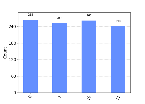
Let’s run this on the QiskitCircuitSimulator backend:

>>> from qutip_qip.qiskit import QiskitCircuitSimulator
>>> backend = QiskitCircuitSimulator()
>>> job = backend.run(circ)
>>> result = job.result()

The result object inherits from the qiskit.result.Result class. Hence, we can use it’s functions like result.get_counts() as required. We can also access the final state with result.data()['statevector'].

>>> result.data()['statevector']
Statevector([0.+0.j, 1.+0.j, 0.+0.j, 0.+0.j], dims=(2, 2))

>>> from qiskit.visualization import plot_histogram
>>> plot_histogram(result.get_counts())

(png, hires.png, pdf)

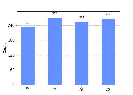
Now, let’s run the same circuit on QiskitPulseSimulator. To use the QiskitPulseSimulator backend, we first need to define the processor on which we want to run the circuit e.g. LinearSpinChain, DispersiveCavityQED etc. We can specify the parameters of those processor and also include noise models. Please refer to the documentation for details.

>>> from qutip_qip.device import LinearSpinChain
>>> processor = LinearSpinChain(num_qubits=2)

>>> pulse_circ = QuantumCircuit(2,2)
>>> pulse_circ.h(0)
>>> pulse_circ.h(1)

While using a pulse processor, we define the circuit without measurements.

Note

The pulse-level simulator does not support measurement. Please use qutip.measure to process the result manually. By default, all the qubits will be measured at the end of the circuit.

>>> from qutip_qip.qiskit import QiskitPulseSimulator

>>> pulse_backend = QiskitPulseSimulator(processor)
>>> pulse_job = pulse_backend.run(pulse_circ)
>>> pulse_result = pulse_job.result()

>>> plot_histogram(pulse_result.get_counts())

(png, hires.png, pdf)

Configurable Options

Qiskit’s interface allows us to provide some options like shots while running a circuit on a backend. We also have provided some options for the qutip_qip backends.

shots

shots is the number of times measurements are sampled from the simulation result. By default it is set to 1024.

An example demonstrating configuring options:

backend = QiskitCircuitSimulator()
job = backend.run(circ, shots=3000)
result = job.result()

We provided the value of shots explicitly, hence our options for the simulation are set as: shots=3000.

Another example:

backend = QiskitCircuitSimulator()
job = backend.run(circ, shots=3000, allow_custom_gate=False)
result = job.result()

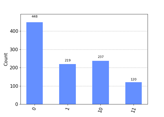
Noise

Real quantum devices are not ideal and are bound to have some amount of noise in them. One of the uses of having the pulse backends is the ability to add noise to our device.

Let’s look at an example where we add some noise to our circuit and see what kind of bias it has on the results. We’ll use the same circuit we used above.

Let’s use the CircularSpinChain processor this time with some noise.

>>> from qutip_qip.device import CircularSpinChain
>>> processor = CircularSpinChain(num_qubits=2, t1=0.3)

If we ran this on a processor without noise we would expect all states to be approximately equiprobable, like we saw above.

>>> noisy_backend = QiskitPulseSimulator(processor)
>>> noisy_job = noisy_backend.run(pulse_circ)
>>> noisy_result = noisy_job.result()

t1=0.3 will cause amplitude damping on all qubits, and hence, 0 is more probable than 1 in the final output for all qubits.

We can see what the result looks like in the density matrix format:

>>> noisy_result.data()['statevector']
DensityMatrix([[ 0.4484772 +0.00000000e+00j,  0.04130281+2.46325222e-01j,
         0.04130281+2.46325222e-01j, -0.13148987+4.53709696e-02j],
       [ 0.04130281-2.46325222e-01j,  0.22120721+0.00000000e+00j,
         0.13909747-1.10349672e-17j,  0.02037223+1.21497634e-01j],
       [ 0.04130281-2.46325222e-01j,  0.13909747+1.10349672e-17j,
         0.22120721+0.00000000e+00j,  0.02037223+1.21497634e-01j],
       [-0.13148987-4.53709696e-02j,  0.02037223-1.21497634e-01j,
         0.02037223-1.21497634e-01j,  0.10910838+0.00000000e+00j]],
      dims=(2, 2))

>>> plot_histogram(noisy_result.get_counts())

(png, hires.png, pdf)