Grover’s Search Algorithm
Grover’s algorithm [7] provides a quadratic speedup for searching an unstructured database of size \(N\). It works by iteratively rotating a quantum state vector toward a “marked” solution state using a phase oracle and a diffusion operator.
Overview
Grover’s algorithm is a fundamental quantum algorithm that finds the unique input to a black-box function that produces a particular output value. The implementation consists of two main components:
The Oracle: A phase oracle that flips the sign of the amplitude for the “marked” states passed by the user.
The Diffusion Operator: This operator flips the current state about its previous state.
The algorithm requires an optimal number of iterations, approximately \(\frac{\pi}{4}\sqrt{\frac{N}{M}}\), where \(N=2^n\) is the size of the search space and \(M\) is the number of marked states.
Constructing the Algorithm
In this module, you can construct the full Grover search circuit using the grover() function. To make the process easier, a utility function grover_oracle() is provided to generate standard phase-flip oracles if the marked states are known.
The grover() function requires the following:
Argument |
Description |
|---|---|
|
A |
|
List of qubit indices (or integer count) to run the search on. |
|
Integer representing the number of marked states \(M\). |
|
Optional integer for manual control over the rotation count. |
|
Optional total number of qubits when searching on a subset of a larger system. |
Example: Searching for Multiple Targets
Let’s simulate a search on 3 qubits (\(N=8\)) where two states are marked: \(|011\rangle\) (index 3) and \(|101\rangle\) (index 5).
First, we import the necessary components and define our search space.
>>> import matplotlib.pyplot as plt
>>> from qutip import basis, tensor
>>> from qutip_qip.algorithms.grover import grover, grover_oracle
>>> n_qubits = 3
>>> marked = [3, 5]
We then use the utility function grover_oracle() to create a phase-flip oracle for our marked states.
>>> oracle = grover_oracle(n_qubits, marked)
Using the grover() function, we construct the full circuit. Since we provide the mandatory num_solutions, the algorithm automatically calculates the optimal number of iterations [7].
>>> qc = grover(oracle, n_qubits, num_solutions=len(marked))
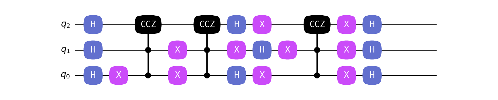
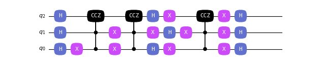
We can also visually render the circuit:
>>> qc.draw()
We can now simulate the circuit by computing the full unitary and applying it to the initial state.
>>> U_grover = qc.compute_unitary()
>>> psi0 = tensor([basis(2, 0)] * n_qubits)
>>> psi_final = U_grover * psi0
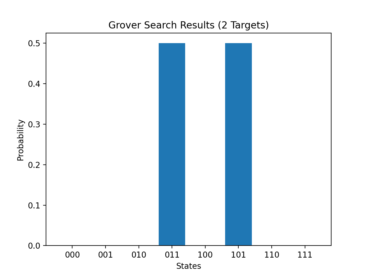
To visualize the results, we calculate the measurement probabilities for all possible states and plot them.
>>> probabilities = [float(abs(psi_final.overlap(basis(2**n_qubits, i)))**2) for i in range(2**n_qubits)]
>>> states = [format(i, f'0{n_qubits}b') for i in range(2**n_qubits)]
>>> plt.bar(states, probabilities)
<...>
>>> plt.title("Grover Search Results (2 Targets)")
Text(...)
>>> plt.xlabel("States")
Text(...)
>>> plt.ylabel("Probability")
Text(...)
>>> plt.show()
